Enhanced Classification of Prostate Cancer Datasets using Supervised Machine Learning Models
1Professor, School of Engineering Technology, Purdue University, USA 2Purdue University and Paavai Engineering College, Nammakkal, India
Author and article information
Cite this as
Sundararajan R, Bensho Sulfick Singh JD. Enhanced Classification of Prostate Cancer Datasets using Supervised Machine Learning Models. J BioData Min. 2026;2(1):1-17. Available from: 10.17352/jbdm.000003
Copyright License
© 2026 Sundararajan R, et al. This is an open-access article distributed under the terms of the Creative Commons Attribution License, which permits unrestricted use, distribution, and reproduction in any medium, provided the original author and source are credited.Abstract
Prostate cancer is one of the most frequently diagnosed cancers among men worldwide and remains a major cause of cancer-related mortality, with over 1.4 million new cases and approximately 375,000 deaths reported annually. Accurate classification of patients into high- and low-risk groups, commonly guided by clinical indicators, such as the Gleason score and prostate-specific antigen (PSA), is essential for early diagnosis and effective treatment planning. In this study, five publicly available datasets were analyzed using seven supervised machine learning models, including Logistic Regression, Naïve Bayes, Decision Tree, Support Vector Machine (SVM), K-Nearest Neighbors (KNN), Random Forest, and Extreme Gradient Boosting (XGBoost). Model performance was evaluated using accuracy, precision, recall, and F1-score. Sensitivity, specificity, the area under the ROC curve (AUC) with 95% confidence intervals, the Brier score and a simple majority-class baseline were also reported. Random Forest showed the highest accuracy of 92.00% with 100% recall in Prostate Adenocarcinoma Dataset 1, while XGBoost showed the highest accuracy of 72.50% in Dataset 2, XGBoost, the highest accuracy of 87.66% in Dataset 3, KNN, the highest accuracy of 90.02% in Dataset 4, and again Random Forest, the highest accuracy of 87.50% with 100% recall in Dataset 5. Across all the datasets, ensemble-based approaches, such as Random Forest and XGBoost consistently demonstrate more balanced and reliable performance, particularly in maintaining high recall, which is critical for minimizing false negatives in medical diagnosis. These findings highlight the effectiveness of machine learning models for prostate cancer risk classification and emphasize the importance of selecting appropriate models based on dataset characteristics. Before any clinical use, the models need further validation.
Introduction
Prostate cancer is the most frequently diagnosed cancer among men in the world, and in the United States, it accounts for nearly 30% of all male cancer cases, with an estimated 313,780 new cases and 35,770 deaths projected for 2025 [1]. It ranks as the second-leading cause of cancer-related death in men, behind only lung cancer, underscoring the ongoing need for accurate and timely risk assessment. Prostate cancer can be classified as high- and low-risk, based on Gleason score and prostate-specific antigen (PSA) level [2]. Gleason score is a grading system that tells doctors how aggressive prostate cancer is by looking at the tissue samples under a microscope. PSA is a protein produced by the prostate gland and is commonly used as a biomarker for prostate cancer screening. In clinical practice, PSA levels below 4 ng/mL are generally considered normal, while levels between 4–10 ng/mL are regarded as borderline or moderately elevated. PSA levels above 10 ng/mL are associated with a higher risk of prostate cancer and may indicate aggressive disease. However, elevated PSA levels can also occur due to non-cancerous conditions, such as benign prostatic hyperplasia or prostatitis, making PSA a sensitive but not highly specific indicator. The low specificity of PSA can lead to unnecessary biopsy [3].
Low risk prostate cancer is that which has not grown outside of the prostate, with low Gleason score and low PSA level [2]. High risk prostate cancer is that where the tumor has grown outside the prostate, with high Gleason score and high PSA level. Table 1 shows the classification of prostate cancer cases into different risk groups based on the International Society of Urological Pathology (ISUP) Grade Group and corresponding Gleason scores. Each risk category is defined using specific score ranges that indicate the characteristics of the tumor [4]. Figure 1 shows the clinical distinction between low/intermediate-favorable risk and intermediate-unfavorable/high-risk prostate cancer [5].
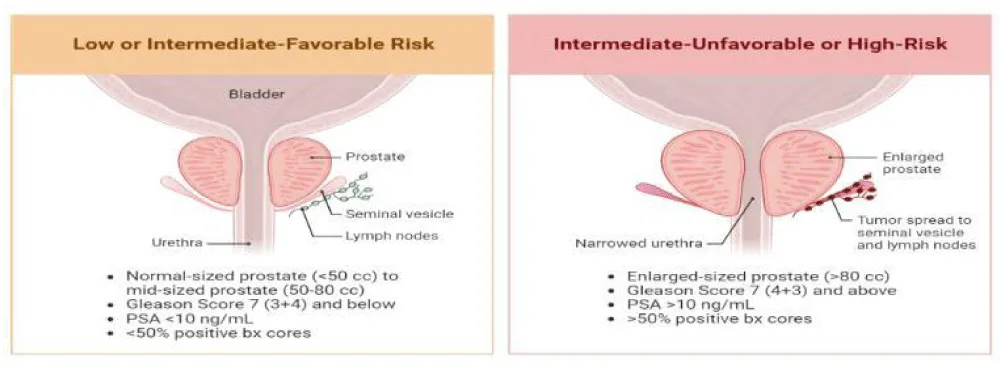
Early detection and accurate risk assessment are essential for improving treatment outcomes, reducing mortality rates, and enabling timely clinical intervention. Traditional diagnostic approaches, such as PSA testing, digital rectal examination, biopsy analysis, and clinical imaging are commonly used to identify prostate cancer [6]. Although these techniques play an important role in medical diagnosis, they may sometimes lead to delayed detection, overdiagnosis, or inaccurate risk stratification due to the complexity of clinical and biological factors involved in cancer progression. As a result, there is a growing need for more reliable and data-driven approaches that can assist clinicians in identifying high-risk patients more accurately.
With the rapid growth of biomedical data and advances in computational technologies, machine learning (ML) models have emerged as powerful tools for analyzing complex medical datasets [7]. ML algorithms can identify hidden patterns and relationships within clinical data that may not be easily detected using conventional statistical methods. These techniques have been successfully applied in various medical applications, including disease prediction, medical imaging analysis, and cancer diagnosis. In supervised machine learning, a model is trained using labeled data, where each input sample is associated with a known output. The objective is to learn a mapping function that accurately relates input features to their corresponding target labels, enabling the model to make predictions on unseen data. Thus, in supervised learning, the model is provided with a training dataset consisting of input-output pairs. During the training phase, the algorithm analyzes the relationship between the input features and the target variable and iteratively adjusts its internal parameters to minimize the prediction error. This process continues until the model achieves an optimal representation of the data. Once trained, the model applies the learned patterns to new data for prediction [7].
Several studies have been conducted on prostate cancer classification. For example, Rustam and Angie [6] proposed a prostate cancer classification framework using Random Forest (RF) and Support Vector Machine (SVM) algorithms to analyze clinical datasets and evaluate prediction performance. Their results demonstrated that ensemble learning methods, such as Random Forest can provide improved classification accuracy compared to traditional models by combining multiple decision trees to enhance predictive stability. Kourou et al. reviewed the application of SVM, Decision Tree (DT), and Neural Networks in cancer prediction and prognosis. Their study highlighted that machine learning models can improve accuracy by approximately 15-20% compared to traditional models [8].
Similarly, Xiao et al. applied the RF algorithm to predict prostate cancer using ultrasound findings and PSA levels [9]. Their study demonstrated that RF effectively handled complex clinical features and improved prediction accuracy in prostate cancer diagnosis, highlighting the usefulness of ensemble learning methods in medical applications. Lay et al. investigated prostate cancer detection using multiparametric magnetic resonance imaging (MRI) data and RF models with instance weighting techniques. Their approach improved diagnostic performance by incorporating imaging features and addressing class imbalance in the dataset [10].
Support Vector Machines have been widely used in biomedical classification tasks due to their ability to construct optimal decision boundaries in high-dimensional datasets. Cortes and Vapnik introduced the concept of support-vector networks, which maximize the margin between data points of different classes and improve classification performance in complex datasets [11]. Özhan and Yagin proposed a machine learning framework for prostate cancer classification based on clinical biomarkers and patient attributes. Their study demonstrated that Random Forest and other supervised learning models can effectively classify cancer cases using biomedical indicators and provide reliable predictive performance [12].
Comparative studies have also evaluated the performance of SVM and RF for prostate cancer prediction. Sakouvogui conducted a comparative classification analysis of prostate cancer datasets using these algorithms and reported that both models achieved strong classification performance, with RF showing improved robustness for complex datasets [13]. Zheng et al. developed machine learning-based models to enhance prostate cancer prediction and reported improved performance over conventional approaches, highlighting the effectiveness of data-driven techniques in clinical decision support [14].
XGBoost, introduced by Chen and Guestrin, is a scalable end-to-end tree boosting system designed to achieve state-of-the-art performance on a wide range of machine learning tasks [11]. The algorithm builds an ensemble of decision trees sequentially, where each successive tree is trained to correct the residual errors of the previous trees using a regularized learning objective that balances predictive accuracy with model complexity, thereby reducing the risk of overfitting. Its efficiency stems from a sparsity-aware algorithm for handling missing or sparse data, a weighted quantile sketch that enables approximate tree learning on large datasets, and system-level optimizations such as cache-aware access patterns, data compression, and out-of-core computation, which together allow the model to scale to datasets containing billions of examples using comparatively few computational resources. These characteristics, combined with its strong empirical performance, have made XGBoost a widely adopted algorithm in biomedical and clinical prediction tasks, including cancer risk classification problems similar to the one addressed in this study.
Table 2 summarizes a partial list of previous studies indicating the number of datasets, evaluation metrics, machine learning models, and additional analysis.
Unlike most earlier studies, which used only one dataset (Table 2), this study compares seven models across five public datasets and reports accuracy, sensitivity, specificity and AUC, showing how model performance changes between datasets. The research question of this study is: how well can standard supervised machine learning classifiers classify high- and low-risk prostate cancer using clinical and genomic data from the five public datasets used?
Methods
Datasets
Five prostate cancer datasets [18-22], publicly available at CBioportal were utilized to evaluate the performance of various machine learning models for risk classification, using seven supervised ML models. These datasets contain clinical and diagnostic attributes relevant to prostate adenocarcinoma. Prostate adenocarcinoma (PD) Dataset 1 consists of 123 samples [18], Dataset 2 has 240 samples [19], Dataset 3 is the largest with 2,069 samples [20], Dataset 4 contains 104 samples [21], and Dataset 5 contains 494 samples [22]. Each dataset includes features, such as clinical measurements, tumor characteristics, and diagnostic indicators, which are used to classify patients into high-risk and low-risk categories. These datasets vary in size, feature distribution, and complexity, providing a comprehensive evaluation environment for comparing different machine learning algorithms. The diversity across datasets enables analysis of model robustness and generalization capability in prostate cancer risk classification.
Table 3 gives the details of the five datasets, including the number of samples before and after cleaning, the number of low-risk and high-risk patients, and the population.
No patient IDs are shared in these five datasets. Each dataset was trained and tested separately, so any overlap of samples or batch effects between datasets does not mix within one model.
Dataset description
Table 4 summarizes the clinical predictors used in this study [18-22]. These features include patient demographics, tumor characteristics, and molecular attributes that serve as input variables for the machine learning models.
Dataset representation
The dataset consists of feature vectors representing patient data, where each sample is labeled as either low-risk (0) or high-risk (1) prostate cancer. This forms a supervised learning dataset of input-output pairs (𝑥𝑖, 𝑦𝑖) [ 23]. Let the dataset be represented as:
X = {x1, x2, ..., xn},
where, each sample xi represents a feature vector describing clinical and tumor attributes of a patient. Each sample has a corresponding label:
𝑦𝑖 ∈ 0,1
where, 𝑦𝑖 = 0 represents low-risk (non-aggressive) prostate cancer, 𝑦𝑖 = 1 represents high-risk (aggressive) prostate cancer.
Thus, the complete dataset can be expressed as:
where, 𝑥𝑖 denotes the feature vector for the ith patient, 𝑦𝑖 represents the class label associated with that patient, N is the total number of patient samples in the dataset.
The high-risk and low-risk groups were defined using the Gleason score (ISUP Grade Group) for each dataset, as shown in Table 5. Full clinical risk groups, such as the NCCN groups, combine the Gleason score, PSA and tumour stage [2]. The Gleason score / Grade Group was used because it is available in all datasets and is the main factor in these risk groups.
Data preprocessing
Data preprocessing was performed to ensure data quality, consistency, and suitability for machine learning analysis. This process involved handling missing values, removing incomplete records, and selecting relevant features for classification. After preprocessing, Prostate Adenocarcinoma (PD) dataset 1 was reduced to 98 samples from 123, dataset 2 to 197 samples from 240, dataset 3 to 1278 samples from 2069, dataset 4 retained all 104 samples, and dataset 5 was reduced to 197 samples from 494. The cleaned datasets were then used for model training and evaluation (80-20 split). Before training the machine learning models, the dataset is preprocessed to ensure data quality and consistent feature representation [23]. The preprocessing steps are described as follows:
Handling missing values
Any missing or incomplete values present in the datasets were addressed through appropriate data cleaning procedures. Records with insufficient or inconsistent data were removed to maintain dataset reliability. Rows with a missing Gleason score were removed, and other missing numeric values were filled with the median of each feature [21].
Feature standardization
To ensure that all numerical features contribute equally to the model training process, feature standardization was applied using z-score normalization [23]:
𝑧 = (𝑥 – μ)/σ,
where, 𝑧 represents the standardized value of the feature after normalization, 𝑥 denotes the original value of the feature before normalization, μ represents the mean (average) value of that feature across all samples in the dataset, σ denotes the standard deviation of the feature, which measures the spread of the data values around the mean. Standardization ensures that features with larger numerical ranges do not dominate features with smaller ranges during model training.
Categorical variables were converted to numbers, and some skewed variables (such as PSA, mutation count and TMB) were log-transformed. The mean and standard deviation used for standardization were calculated from the training data only and then applied to the test data.
Train-test split
After preprocessing, Datasets 1, 2, 3 and 5 were divided into training and testing subsets using a stratified 80%–20% split. Hyperparameters were tuned with grid search and 5-fold cross-validation on the training data only, and the test set was used once for the final evaluation. Dataset 4 is small (only 104 patients), so 5-fold cross-validation repeated 20 times was used. A random seed of 42 was used for all splits and models. The training set was used to train the machine learning models, while the testing set was used to evaluate their predictive performance [23]. The training and testing sizes are given in Table 6.
Class imbalance and patient separation
SMOTE oversampling was applied to the training data only, and class weights were used for Logistic Regression, Decision Tree, Random Forest and SVM. The test data were never resampled. Each patient appears only once in each dataset, so no patient is in both the training and test sets.
Machine learning workflow
Figure 2 shows the machine learning workflow of the prostate cancer risk classification. The process begins with the collection of five prostate cancer datasets, containing relevant clinical information. In the data preparation stage, the datasets are loaded, and relevant clinical features are selected. The data is then cleaned and organized to ensure consistency and suitability for further analysis. Following this, data preprocessing is performed, which includes handling missing values, applying feature scaling and normalization, and splitting the dataset into training and testing sets using an 80:20 ratio.
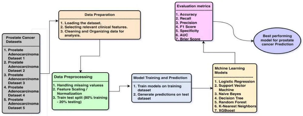
Next, in the model training and prediction phase, seven supervised machine learning models were trained using the training dataset, and predictions are generated on the test dataset. The seven models considered include Logistic Regression (LR), (SVM), Naïve Bayes (NB), Decision Tree (DT), RF, K-Nearest Neighbors (KNN), and XGBoost.
The performance of each model is evaluated using standard evaluation metrics, including accuracy, precision, recall, and F1-score. These metrics provide a comprehensive assessment of model effectiveness, particularly in distinguishing between high-risk and low-risk prostate cancer cases. Finally, based on the evaluation results, the best-performing model is identified for prostate cancer prediction. This workflow ensures a systematic and reliable approach to analyzing clinical datasets and selecting the most suitable machine learning model for risk classification.
Choice of the machine learning models
These seven models were selected based on their effectiveness in handling classification problems and clinical datasets [4]. In this study, the number of decision trees in the RF was set to 150 to balance accuracy and speed. Using more trees generally improves the model’s predictions, but after a certain point, adding more trees (200 trees) does not make a big difference (same accuracy) and only increases computation time. On the other hand, using too few trees (100 trees) can lead to unstable and less accurate results (44.00%). Therefore, 150 trees were chosen as a suitable number that gives good performance while keeping the model efficient [7].
Evaluation metrics
Model performance was evaluated using four standard classification metrics, accuracy, precision, recall, F1 score. Specificity, AUC and the Brier score were also added. Accuracy measures the overall proportion of correctly classified samples among all predictions. It reflects how often the model correctly predicts both positive and negative cases, and is given by,
where, TP represents the number of true positive predictions, TN represents the number of true negative predictions, FP represents the number of false positive predictions and FN represents the number of false negative predictions [24].
Precision measures the proportion of correctly predicted positive samples among all predicted positive samples. It indicates the reliability of positive predictions made by the model, given by,
Recall measures the ability of the model to correctly identify actual positive samples. It represents the proportion of true positive cases detected by the classifier, given by,
F1 score is the harmonic mean of precision and recall. It provides a balanced measure of classification performance when both false positives and false negatives are important, and is given by,
In medical diagnosis, recall is particularly important, as failing to identify aggressive cancer cases can lead to delayed treatment.
Specificity measures the ability of the model to correctly identify low-risk patients [25]. It is calculated as:
𝑆𝑝𝑒𝑐𝑖𝑓𝑖𝑐𝑖𝑡𝑦 = 𝑇𝑁/(𝑇𝑁 + 𝐹𝑃).
ROC curve
The area under the ROC curve (AUC) measures how well the model separates high-risk from low-risk patients across all decision thresholds. An AUC of 0.5 means no better than chance, and 1.0 means perfect separation. The 95% confidence interval of the AUC was calculated by bootstrapping the test set (2,000 resamples); for Dataset 4 it was taken from the spread across the cross-validation folds [26].
TPR (true positive rate)= 𝑇𝑃/(𝑇𝑃 + 𝐹𝑁)
FPR (false positive rate)= 𝐹𝑃/(𝐹𝑃 + 𝑇𝑁)
Brier score
The Brier score measures calibration, which is how close the predicted probabilities are to the actual outcomes. It ranges from 0 to 1, and lower values are better. Calibration curves were also plotted. A simple baseline that always predicts the larger class was included for comparison, as accuracy alone can be misleading when the classes are imbalanced [27].
Confusion matrix
A confusion matrix is used to evaluate the performance of a classification model by comparing actual and predicted labels. The test samples (20%) from the 80-20 split are used in the confusion matrix to calculate the actual and predicted labels (for Dataset 4, the out-of-fold predictions for all 104 patients from cross-validation are used) [28]. Each cell also reports the row-wise percentage, calculated as the cell count divided by the total number of actual samples in that row, expressed as a percentage. This shows what proportion of each true class was classified into each predicted category, with the two percentages in a row summing to 100%.
Heatmap
A heatmap is a data visualization tool that depicts values for a main variable of interest across two axis variables as a grid of colored squares. The axis variables are divided into ranges like a chart or histogram, and each cell’s color indicates the value of the main variable in the corresponding cell range [29].
Results
Prostate adenocarcinoma dataset 1
Figure 3a shows the accuracies of the seven models for PD dataset 1, demonstrating the varying levels of predictive performance. RF produced the highest accuracy at 92%, followed by LR at 88% and XGBoost at 86.96%. The comparatively lower performance of KNN and DT suggests the presence of nonlinear and noisy patterns within the dataset.
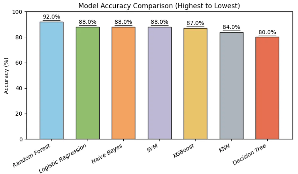
Table 7 lists the model performance of all the four metrics. RF predicted the best overall performance with the highest accuracy (92%) and F1-score (95.65%), along with 100% recall, indicating its strong ability to correctly identify high-risk cases. LR, NB, and SVM also performed well with equal accuracy (88%) and recall (100%), but slightly lower precision compared to RF. XGBoost showed a competitive accuracy of 86.96% with strong recall (95.00%), close behind the top traditional models. KNN showed moderate performance, while DT had the lowest accuracy and F1-score among all models. Overall, the results highlight that ensemble methods like RF provide more reliable and balanced performance for prostate cancer classification.
The occurrence of 100% recall in LR, NB, SVM, and RF indicates that these models successfully identify all high-risk prostate cancer cases without any false negatives. This is particularly important in medical diagnosis, where missing a cancer case can have serious consequences. However, achieving perfect recall often comes at the cost of reduced precision, as the model may classify some low-risk cases as high-risk, leading to an increase in false positives. Therefore, while high recall reflects strong sensitivity, it must be considered alongside precision and F1-score to evaluate overall model performance.
DT demonstrates comparatively lower recall (86.36%) despite having relatively high precision (90.47%), indicating that it misses a significant number of high-risk cases, which is undesirable in medical diagnosis. Overall, it can be seen that those models with higher recall are more suitable for medical applications where minimizing false negatives is critical. Among all models, RF provides the most reliable and balanced performance for prostate cancer risk classification for dataset 1.
Confusion matrices
Figure 3b shows the confusion matrices of the machine learning models in terms of TN, FP, FN, and TP for high- and low-risk prostate cancer classification. For the RF model, the values are 1 TN (50.0%), 1 FP (50.0%), 0 FN (0.0%), and 18 TP (100.0%), indicating excellent performance with zero false negatives and correct identification of all high-risk cases. The LR model shows 2 TN (100.0%), 0 FP (0.0%), 7 FN (38.9%), and 11 TP (61.1%), indicating higher false negatives, which reduces its effectiveness in identifying high-risk cases despite having no false positives. The NB model achieved 0 TN (0.0%), 2 FP (100.0%), 0 FN (0.0%), and 18 TP (100.0%), demonstrating 100% recall with no missed high-risk cases, but with false positives indicating misclassification of low-risk cases. For SVM, the values are 2 TN (100.0%), 0 FP (0.0%), 4 FN (22.2%), and 14 TP (77.8%), showing moderate performance with some missed high-risk cases.
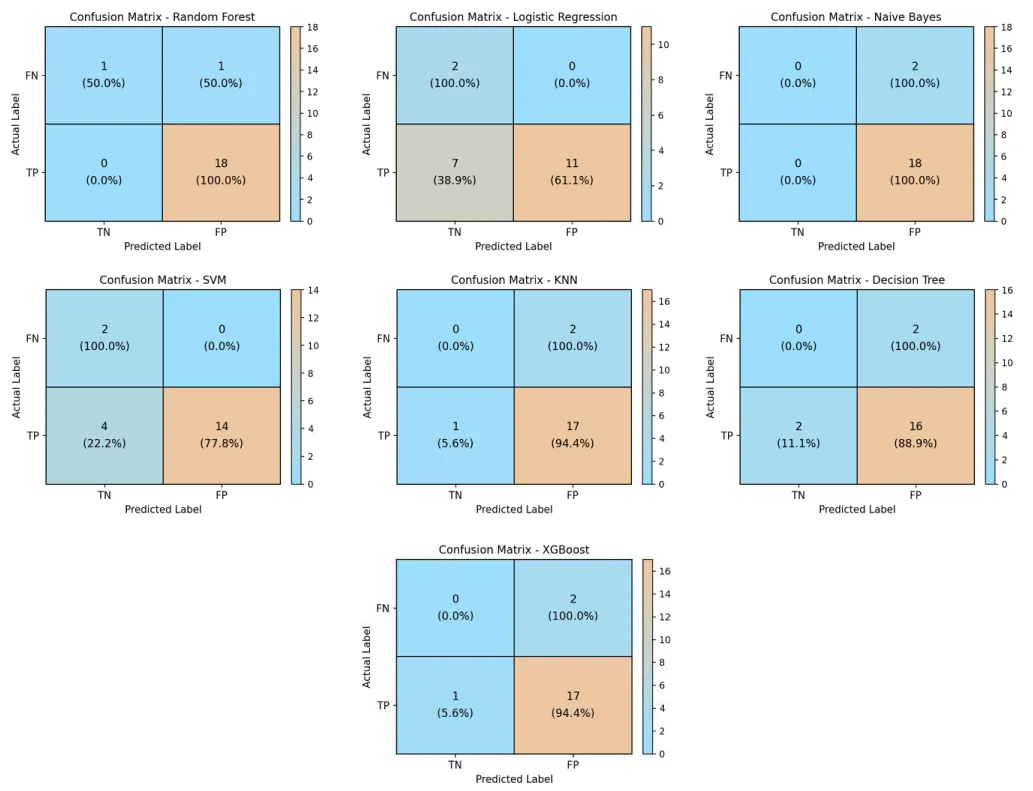
The KNN model shows 0 TN (0.0%), 2 FP (100.0%), 1 FN (5.6%), and 17 TP (94.4%), indicating high recall with minimal false negatives but some false positives. The DT model has 0 TN (0.0%), 2 FP (100.0%), 2 FN (11.1%), and 16 TP (88.9%), demonstrating comparatively lower performance due to higher false negatives. Finally, the XGBoost model shows 0 TN (0.0%), 2 FP (100.0%), 1 FN (5.6%), and 17 TP (94.4%), indicating strong recall with only one missed high-risk case, although it did not correctly classify any of the low-risk cases in this split.
Overall, RF provides the best performance with zero false negatives. NB also has zero false negatives, but it reached 100% recall only because it predicted every patient as high-risk, giving 0% specificity, so it is not considered one of the best models. XGBoost also performs strongly with only one false negative. However, NB produces more false positives, reducing precision. LR and SVM show higher false negatives, making them less suitable for medical diagnosis. KNN provides balanced performance, while Decision Tree shows comparatively lower effectiveness.
These results emphasize the importance of minimizing false negatives in clinical applications, as missing high-risk prostate cancer cases can lead to delayed diagnosis and treatment.
Heatmap analysis of all the models performance
Figure 4 shows the heatmap for performance of seven machine learning models across the five different prostate cancer datasets using accuracy, precision, recall, and F1-score as evaluation metrics. As indicated before, for Prostate Adenocarcinoma Dataset 1, RF achieved the highest accuracy of 92% along with 100% recall, indicating its strong ability to correctly identify all high-risk cases, while LR, NB, and SVM also achieved 100% recall but with slightly lower precision. For Prostate Adenocarcinoma Dataset 2, overall performance drops significantly, indicating higher complexity; XGBoost achieved the highest accuracy of 72.5, followed by KNN of 68%, while RF provides a better balance with higher F1-score, and NB shows very low recall despite high precision. In Dataset 3, DT and RF, both achieved the highest accuracy of 84.38%, with RF attaining the highest F1-score (91.11%), demonstrating a balanced classification performance. In Dataset 4, KNN achieved the highest accuracy of 90.02%, while RF again provides strong overall balance with high recall and F1-score, making it reliable for clinical prediction.
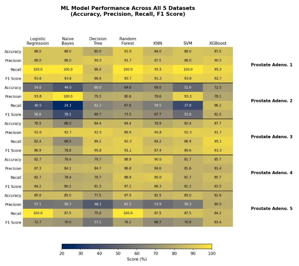
Sentation of model performance across datasets
In Dataset 5, RF showed the highest accuracy of 87.50% with 100% recall, indicating excellent detection of high-risk cases, while LR also showed 100% recall, but with lower precision. Across the five datasets, XGBoost also demonstrated competitive and often leading performance, achieving the highest accuracy on Datasets 2 and 3. Across all datasets, RF consistently demonstrated the most balanced and reliable performance, particularly in maintaining high recall, which is critical in medical diagnosis to minimize false negatives.
Confusion matrices
Dataset 2: Figure 5a shows the confusion matrices for dataset 2. For the KNN model, the values are 4 TN (36.4%), 7 FP (63.6%), 8 FN (27.6%), and 21 TP (72.4%), indicating a relatively high number of false negatives and false positives, which reduces its overall reliability. The RF model achieved 6 TN (54.5%), 5 FP (45.5%), 10 FN (34.5%), and 19 TP (65.5%), demonstrating moderate performance but with a noticeable number of missed high-risk cases. Similarly, the DT model shows 6 TN (54.5%), 5 FP (45.5%), 10 FN (34.5%), and 19 TP (65.5%), indicating comparable performance to RF, but without improvement in reducing false negatives. The LR model has 9 TN (81.8%), 2 FP (18.2%), 16 FN (55.2%), and 13 TP (44.8%), showing lower false positives but a significantly higher number of false negatives, which negatively impacts its effectiveness in detecting high-risk cases.
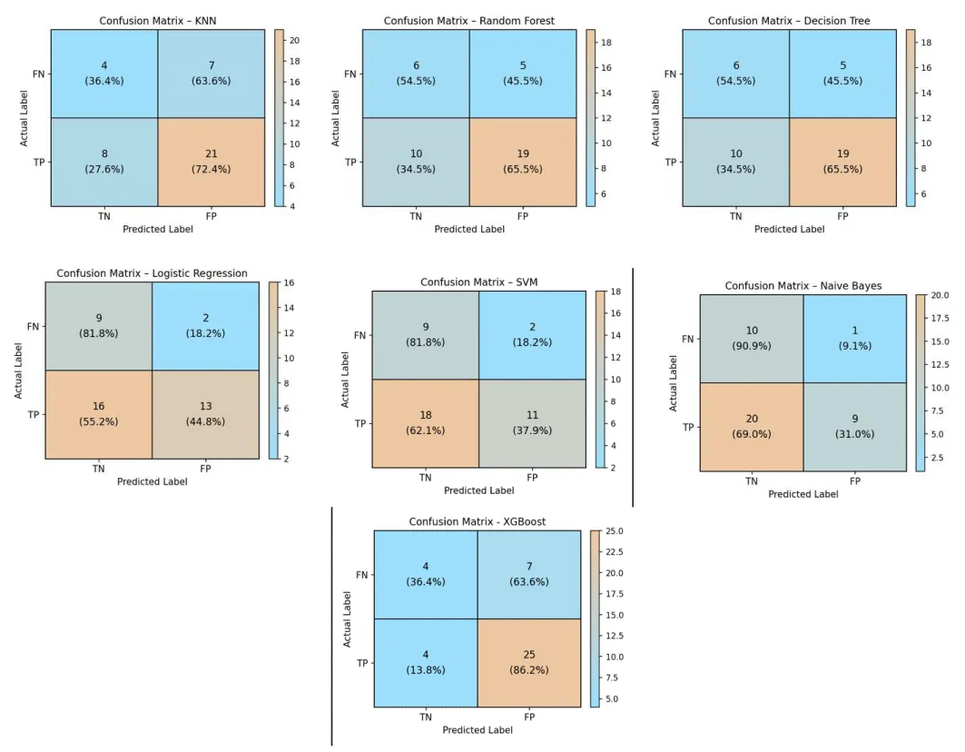
For SVM, the values are 9 TN (81.8%), 2 FP (18.2%), 18 FN (62.1%), and 11 TP (37.9%), indicating poor sensitivity due to a high number of missed high-risk cases. The NB model shows 10 TN (90.9%), 1 FP (9.1%), 20 FN (69.0%), and 9 TP (31.0%), demonstrating the weakest performance with the highest number of false negatives, despite having minimal false positives. The XGBoost model shows 4 TN (36.4%), 7 FP (63.6%), 4 FN (13.8%), and 25 TP (86.2%), achieving the highest number of true positives and the fewest false negatives among all models on this dataset.
Overall, all models exhibit increased false negatives in this dataset, indicating difficulty in identifying high-risk prostate cancer cases. XGBoost provides the most balanced result on this dataset, with the fewest false negatives (4) and the highest number of true positives (25). Among the remaining models, RF and DT provided relatively more balanced performance, while LR, SVM, and NB showed reduced sensitivity.
These results highlight the complexity and imbalance, where achieving high recall is challenging. The findings emphasize the need for improved models or techniques to reduce false negatives, as missing high-risk cases can have serious clinical consequences.
Dataset 3: Figure 5b shows the confusion matrices for dataset 3. For the DT model, the values are 18 TN (52.9%), 16 FP (47.1%), 24 FN (10.8%), and 198 TP (89.2%). This indicates a good overall performance with a high number of correctly identified high-risk cases, although some false negatives are present. The RF model shows 11 TN (32.4%), 23 FP (67.6%), 17 FN (7.7%), and 205 TP (92.3%). This indicates strong performance with the highest number of true positives, demonstrating its effectiveness in identifying high-risk patients, although it produces slightly more false positives. For the SVM, the values are 18 TN (52.9%), 16 FP (47.1%), 29 FN (13.1%), and 193 TP (86.9%). This shows good precision, but a higher number of false negatives compared to RF, indicating that some high-risk cases are missed. The KNN model has 15 TN (44.1%), 19 FP (55.9%), 35 FN (15.8%), and 187 TP (84.2%). This indicates moderate performance, with a relatively higher number of false negatives, reducing its effectiveness in identifying all high-risk patients.
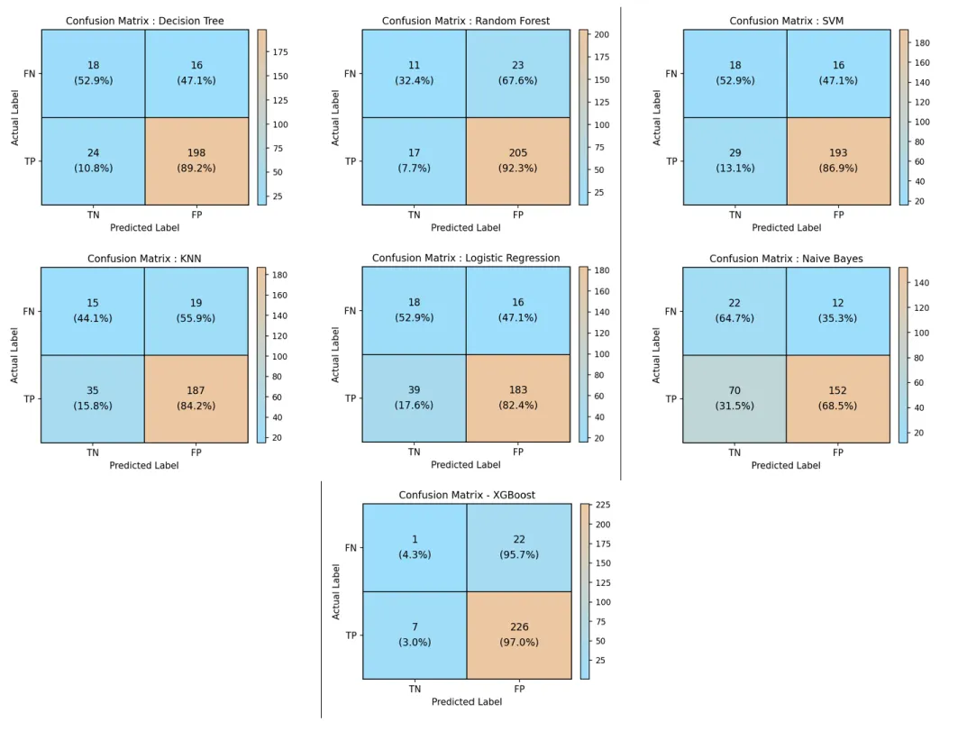
For LR, the values are 18 TN (52.9%), 16 FP (47.1%), 39 FN (17.6%), and 183 TP (82.4%). This suggests that while the model maintains reasonable classification, it misses a significant number of high-risk cases due to higher false negatives. The NB model shows 22 TN (64.7%), 12 FP (35.3%), 70 FN (31.5%), and 152 TP (68.5%). This indicates the weakest performance among all models, with a very high number of false negatives, meaning many high-risk cases are not correctly identified. Finally, the XGBoost model shows 1 TN (4.3%), 22 FP (95.7%), 7 FN (3.0%), and 226 TP (97.0%), achieving fewer false negatives and more true positives than RF, indicating stronger sensitivity for identifying high-risk cases.
Overall, these confusion matrices indicate that XGBoost provides the strongest performance with the highest true positives (226) among all models, while also achieving the lowest false negative count (7), well below RF’s 17. RF also performed well, with the highest true positives and relatively low false negatives. DT and SVM also showed strong performances, while KNN and LR demonstrate moderate effectiveness. NB performed the worst, with high false negative rate. These results further confirm that models with lower false negatives are more suitable for medical applications, as missing high-risk prostate cancer cases can lead to serious clinical consequences.
XGBoost was run separately from the other six models with a different random split, which is why its class totals (23 low-risk / 233 high-risk) differ from the other models (34 / 222). Its very low specificity (1 TN, 4.3%) shows that it identifies few low-risk patients.
Dataset 4: Figure 5c shows the confusion matrices for dataset 4. They show the predictions for all 104 patients from the same 5-fold cross-validation used for the accuracy. KNN has 91 TN (100.0%), 0 FP (0.0%), 9 FN (69.2%) and 4 TP (30.8%); Random Forest has 82 TN (90.1%), 9 FP (9.9%), 6 FN (46.2%) and 7 TP (53.8%); Logistic Regression has 78 TN (85.7%), 13 FP (14.3%), 6 FN (46.2%) and 7 TP (53.8%); SVM has 83 TN (91.2%), 8 FP (8.8%), 11 FN (84.6%) and 2 TP (15.4%); Decision Tree has 79 TN (86.8%), 12 FP (13.2%), 7 FN (53.8%) and 6 TP (46.2%); Naive Bayes has 72 TN (79.1%), 19 FP (20.9%), 8 FN (61.5%) and 5 TP (38.5%); XGBoost has 89 TN (97.8%), 2 FP (2.2%), 7 FN (53.8%) and 6 TP (46.2%). Because only 13 of the 104 patients are high-risk, the high accuracy is mainly due to correctly identifying low-risk patients; for example, KNN identifies all 91 low-risk patients but only 4 of the 13 high-risk patients.
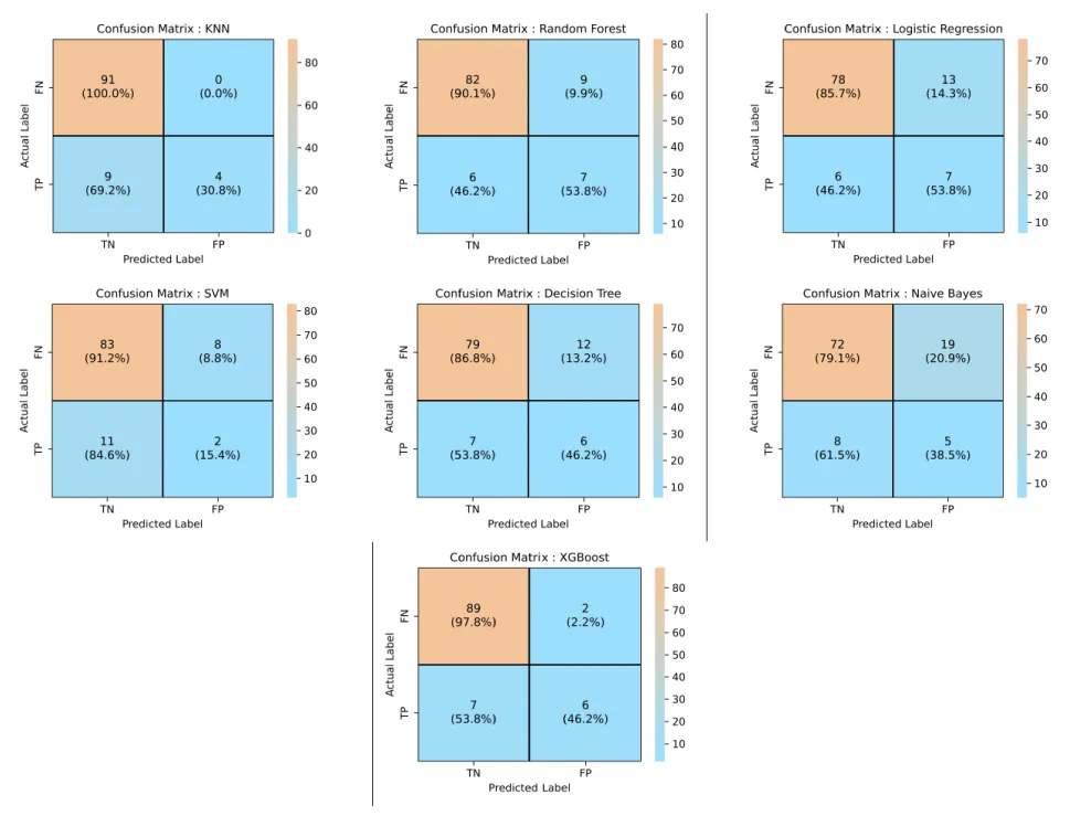
Overall, KNN achieved the highest accuracy (90.02%) on Dataset 4, followed by RF (88.92%). However, because only 13 of the 104 patients are high-risk, all models identify low-risk patients much better than high-risk patients, as shown by the corrected confusion matrices and the high-risk sensitivity values in Table 4d. These results show that accuracy alone can be misleading for this imbalanced dataset.
Dataset 5: Figure 5d shows the confusion matrices for dataset 5. For the RF model, the values are 27 TN (84.4%), 5 FP (15.6%), 0 FN (0.0%), and 8 TP (100.0%), indicating excellent performance with zero false negatives and correct identification of all high-risk cases. The LR model shows 26 TN (81.3%), 6 FP (18.8%), 0 FN (0.0%), and 8 TP (100.0%), also achieving perfect recall with no missed high-risk cases, although with slightly higher false positives compared to RF. For the NB model, the values are 27 TN (84.4%), 5 FP (15.6%), 1 FN (12.5%), and 7 TP (87.5%), indicating strong performance, but with one missed high-risk case. The XGBoost model shows the same confusion matrix values as KNN, with 26 TN (81.3%), 6 FP (18.8%), 1 FN (12.5%), and 7 TP (87.5%), also indicating strong performance with one missed high-risk case.
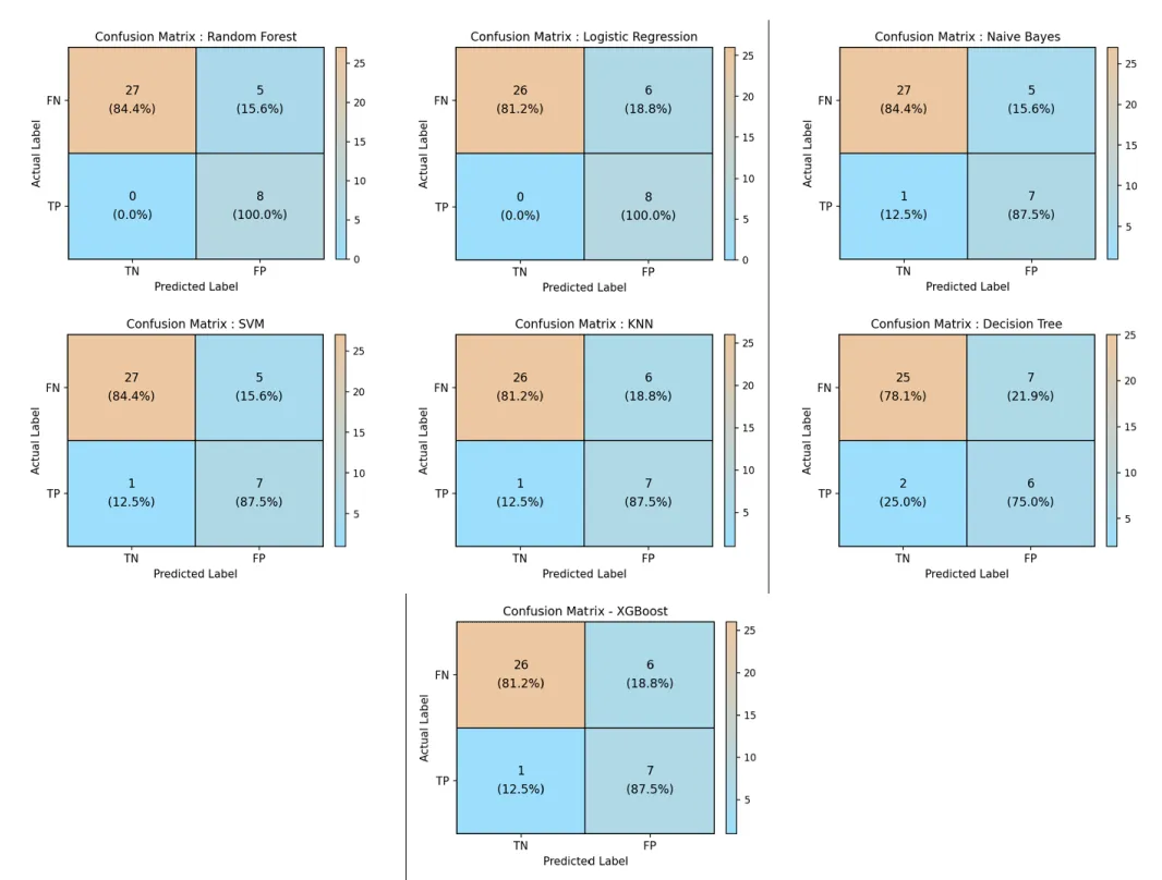
The SVM model has 27 TN (84.4%), 5 FP (15.6%), 1 FN (12.5%), and 7 TP (87.5%), showing similar performance to Naïve Bayes with a small number of false negatives. The KNN model shows 26 TN (81.3%), 6 FP (18.8%), 1 FN (12.5%), and 7 TP (87.5%), indicating moderate performance with slightly higher false positives and one missed high-risk case. Finally, the DT model has 25 TN (78.1%), 7 FP (21.9%), 2 FN (25.0%), and 6 TP (75.0%), demonstrating the lowest performance among all models due to higher false negatives and false positives.
Overall, RF and LR provided the best performance with zero false negatives, where missing high-risk cases must be avoided. NB, SVM, and KNN show moderate performance with minimal misclassification, while DT performs the weakest. These results emphasize the importance of minimizing false negatives in clinical applications, as failure to identify high-risk prostate cancer cases can lead to delayed treatment and serious consequences.
Sensitivity, Specificity, AUC and Calibration
Tables 8a–8e give the sensitivity, specificity, AUC with 95% confidence interval and Brier score for all models, together with the accuracy, precision, recall and F1-score reported above. A baseline that always predicts the larger class is included for comparison. Figures 6a–6e show the ROC curves and Figures 7a–7e show the calibration curves. In Datasets 1 and 4, the baseline reaches high accuracy (about 87–90%) while identifying no low-risk patients, which shows that accuracy alone is not enough and that sensitivity, specificity and AUC should be considered together.
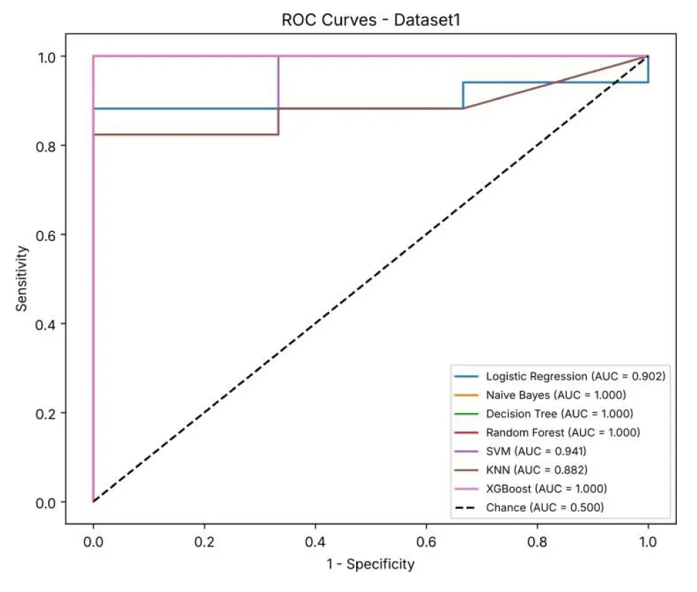
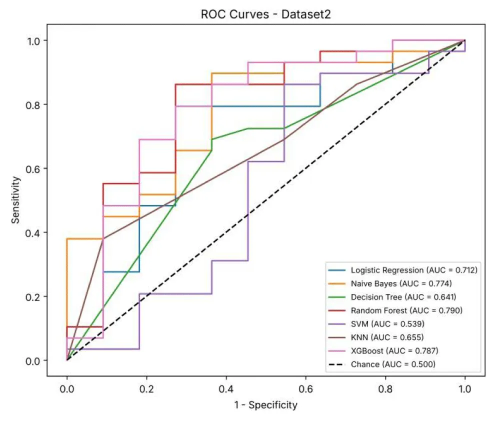
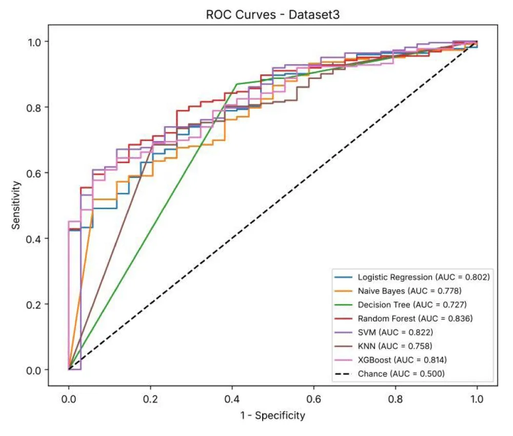
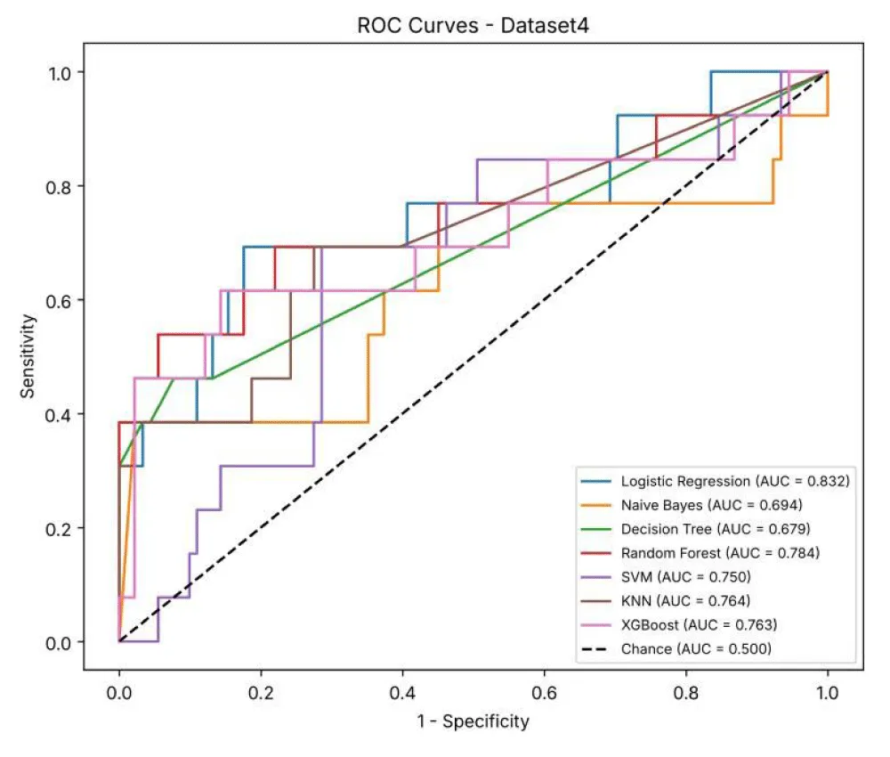
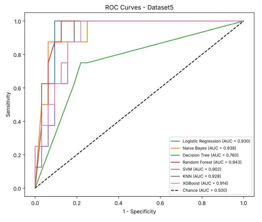
Table 8a shows the sensitivity, specificity, AUC and Brier score of the seven models for Dataset 1, together with the accuracy, precision, recall and F1-score from Table 4. NB, DT, RF and XGBoost reached an AUC of 1.000, but the test set contains only two low-risk patients, so these values should be read with caution. Specificity varies widely, from 0% (NB, DT, KNN and XGBoost) to 100% (LR and SVM), and the baseline that predicts every patient as high-risk already reaches 90.00% accuracy.
Table 8b shows the additional metrics for Dataset 2. RF had the highest AUC (0.790), followed by XGBoost (0.787) and NB (0.774), while SVM had the lowest AUC (0.539). NB had the highest specificity (90.91%) but the lowest recall (24.32%), showing that it identifies low-risk patients well but misses most high-risk patients.
Table 8c shows the additional metrics for Dataset 3, the largest dataset. RF had the highest AUC (0.836), followed by SVM (0.822) and XGBoost (0.814). Because 87% of the test patients are high-risk, specificity is low for all models (4.35–64.71%), and the baseline already reaches 86.72% accuracy.
Table 8d shows the additional metrics for Dataset 4, calculated from the same 5-fold cross-validation repeated 20 times. LR had the highest AUC (0.832), followed by RF (0.784). All models identify low-risk patients well (specificity 83.38–100%), but sensitivity for the high-risk class is low (21.00–60.50%) because only 13 of the 104 patients are high-risk.
In this dataset, most patients are low-risk, so the baseline predicts every patient as low-risk. It never predicts the high-risk class, so its precision cannot be calculated (0/0) and is shown as “–”, and its recall and F1-score are 0%.
Table 8e shows the additional metrics for Dataset 5. RF had the highest AUC (0.943), followed by NB (0.938) and LR (0.930), while DT had the lowest AUC (0.760). Specificity was similar across models (78.12–84.38%), and RF also had the lowest Brier score (0.108), indicating the best agreement between predicted and actual risk.
Figure 6a shows the ROC curves of the seven models for Dataset 1. Each curve plots sensitivity against 1− specificity at different decision thresholds, and the dashed line represents a random classifier (AUC = 0.5). NB, DT, RF and XGBoost reach the top-left corner (AUC = 1.000), while KNN has the lowest AUC (0.882); however, the small test set (20 patients) limits the reliability of these curves.
Figure 6b shows the ROC curves for Dataset 2. RF (AUC = 0.790) and XGBoost (AUC = 0.787) have the curves closest to the top-left corner, showing the best separation of high-risk and low-risk patients. The SVM curve (AUC = 0.539) lies close to the dashed line, meaning it performs only slightly better than chance on this dataset.
Figure 6c shows the ROC curves for Dataset 3. The AUC values range from 0.727 (DT) to 0.836 (RF). The curves are smoother than in the smaller datasets because the test set is larger (256 patients).
Figure 6d shows the ROC curves for Dataset 4, based on the cross-validation predictions for all 104 patients. LR has the highest AUC (0.832), and DT and NB have the lowest (0.679 and 0.694). All curves are above the dashed line, but the wide confidence intervals in Table 4d show that the results are uncertain because there are only 13 high-risk patients.
Figure 6e shows the ROC curves for Dataset 5. RF (AUC = 0.943), NB (0.938), LR (0.930) and KNN (0.928) all have curves close to the top-left corner, showing strong separation of high-risk and low-risk patients. DT has the lowest AUC (0.760).
Figure 7a shows the calibration curves for Dataset 1, which compare the predicted probability of high risk with the actual proportion of high-risk patients; a perfectly calibrated model follows the dashed diagonal line. Most predictions are close to 1.0 because most patients are high-risk, and DT, XGBoost and RF have the lowest Brier scores (0.000–0.009). KNN lies above the line and has the highest Brier score (0.171).
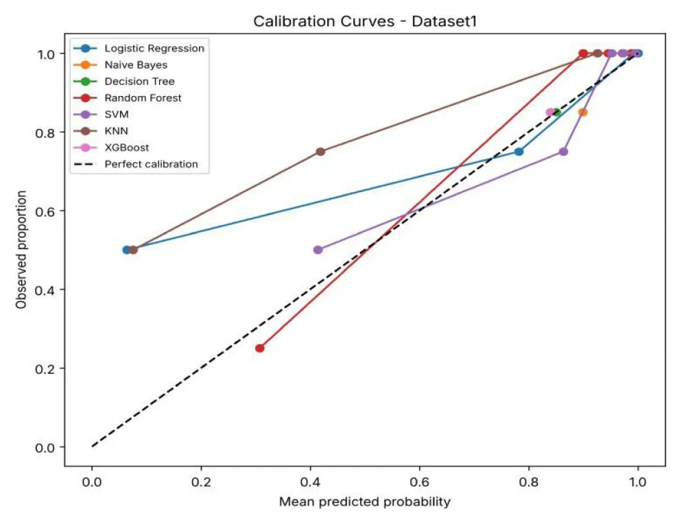
Figure 7b shows the calibration curves for Dataset 2. Most curves lie above the diagonal at low and middle probabilities, meaning that the models often under-estimate the risk of high-risk patients. XGBoost and RF have the lowest Brier scores (0.156 and 0.158), while NB has the highest (0.450).
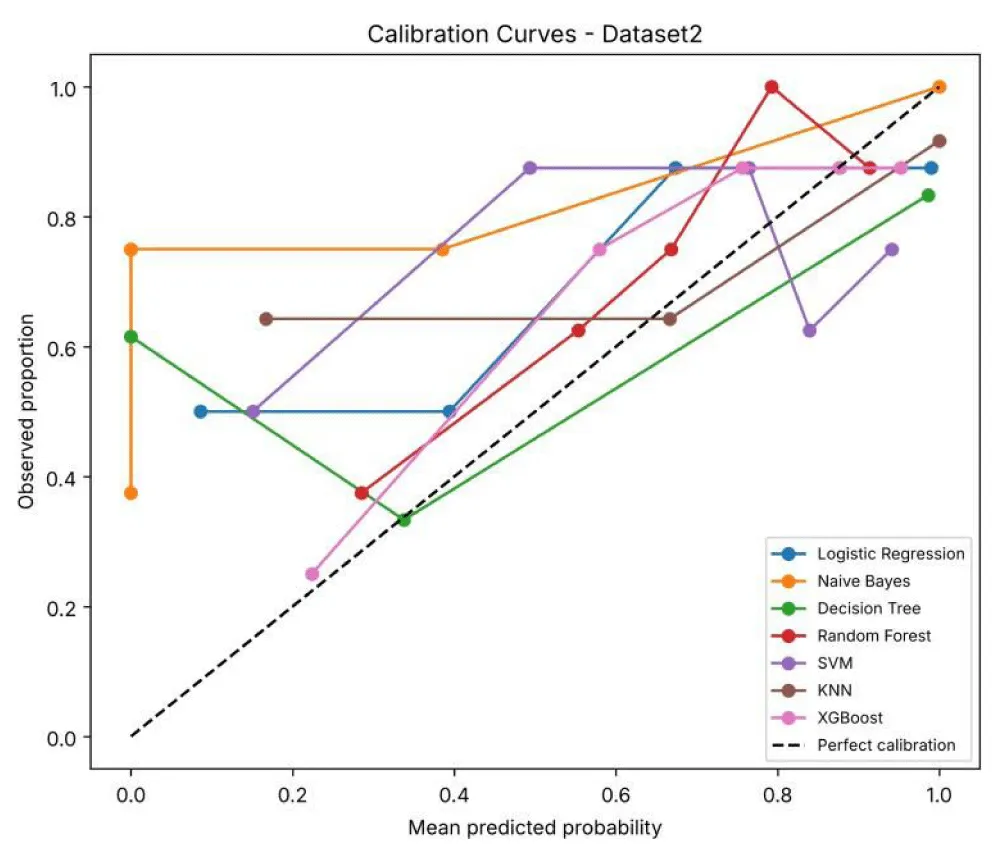
Figure 7c shows the calibration curves for Dataset 3. The curves lie above the diagonal at lower probabilities, meaning that patients given a low predicted risk are still often high-risk, which reflects the large share of high-risk patients in this dataset. RF has the lowest Brier score (0.108) and NB the highest (0.311).
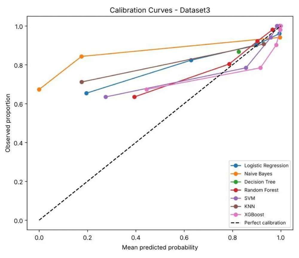
Figure 7d shows the calibration curves for Dataset 4. Most curves lie below the diagonal at higher probabilities, meaning that the models over-estimate the risk of being high-risk. KNN and XGBoost have the lowest Brier scores (0.090 and 0.095), while NB has the highest (0.206).
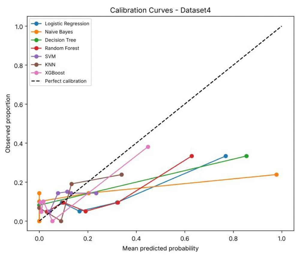
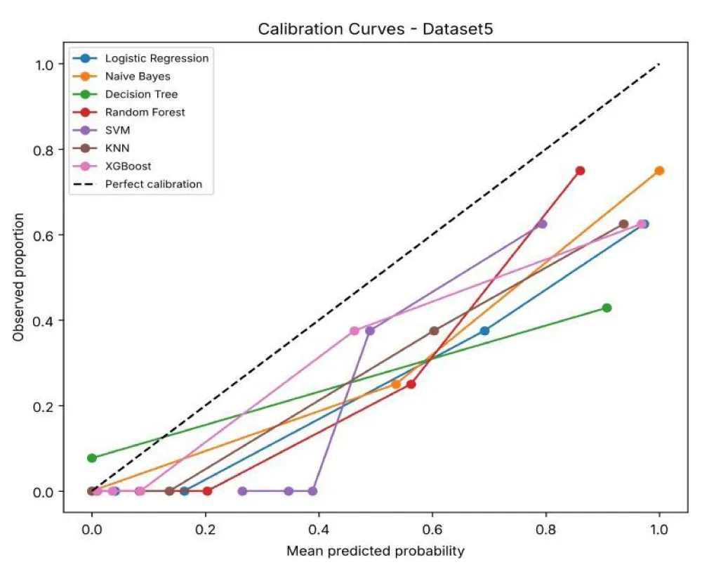
Figure 7e shows the calibration curves for Dataset 5. All curves lie below the diagonal, meaning that the models predict higher risk than is actually observed. RF has the lowest Brier score (0.108) and DT the highest (0.217).
Discussion
A comparison with previous prostate cancer classification model studies (Table 9) shows that Rustam et al.
[6] and Xiao et al. [9], primarily focused on individual clinical datasets and reported strong performance, using models like RF and SVM, achieving accuracies of up to 97.30% and 83.10%, respectively. Similarly, Dubey et al. [16] demonstrated high accuracy using KNN and SVM on the PLCO dataset, while Chen et al. [17] showed balanced performance across LR, DT, RF, and SVM on a clinical biopsy dataset. However, these studies evaluated only one dataset, making it difficult to assess model generalizability. In contrast, our study compares the same seven ML models across five different datasets and reports accuracy, sensitivity, specificity and AUC, which shows how model performance changes between datasets.
Overall, the comparison highlights that while individual models may outperform others on specific datasets, ensemble methods, such as RF and XGBoost consistently provide robust and balanced performance across multiple datasets.
Following the comparative analysis, the variation in model performance across the five datasets can be attributed to differences in dataset size, feature distribution, class balance, and underlying data complexity. In PD Dataset 1, RF achieves the highest accuracy due to its ensemble nature, which combines multiple decision trees to capture complex feature interactions and reduce overfitting. The dataset appears to have well-defined patterns, allowing Random Forest, along with LR, NB, and SVM, to achieve very high recall (100%), indicating clear class separability.
PD Dataset 2 showed the lowest performance across all models, indicating high complexity, noise, or overlapping class distributions. XGBoost performed best in this dataset because it relies on local neighborhood patterns rather than global assumptions. However, models like Logistic Regression and SVM performed poorly due to their inability to effectively separate highly overlapping classes. NB showed high precision but very low recall, meaning it predicts fewer positive cases and misses many high-risk samples, likely due to violation of its independence assumption.
In PD Dataset 3, XGBoost achieved the highest accuracy (87.66%), suggesting that this dataset contains non-linear relationships that tree-based models can effectively capture. RF further improved the performance by reducing variance through ensemble learning. Other models, such as LR and NB performed comparatively lower due to their limitations in handling complex, non-linear feature interactions.
For PD Dataset 4, KNN achieved the highest accuracy (90.02%), indicating that the dataset has strong local structure where similar instances are clustered together. RF also performed well due to its robustness, while LR and SVM show slightly lower performance, suggesting that global decision boundaries are less effective for this dataset.
Finally, in PD Dataset 5, RF again achieved the highest accuracy (87.50%) along with 100% recall. LR, NB, and SVM also achieved competitive performance, indicating relatively balanced and structured data. DT showed comparatively lower performance due to its tendency to overfit when used as a single model without ensemble support.
Overall, the results highlight that no single model performs best across all datasets. Simpler models like LR performed well on linearly separable data, KNN exceled in datasets with strong local patterns, and NB performed well when feature independence approximately holds. However, ensemble models, such as RF and XGBoost consistently provide the most stable and reliable performance due to their ability to handle non-linearity, reduce overfitting. These observations emphasize the importance of selecting models based on dataset characteristics rather than relying on a single approach for all scenarios.
Clinical relevance: The high-risk and low-risk groups used in this study are linked to different treatments. Low-risk patients (Grade Group 1) are usually monitored with active surveillance, while high-risk patients (Grade Group 4–5) usually need surgery or radiotherapy [2]. The models could help flag patients who may need closer attention. However, each dataset was modelled separately, so this study is not an external validation of one model, and the models need external validation before any clinical use.
Limitations: First, the risk groups are based on the Gleason score / Grade Group only and not on full clinical risk groups that also include PSA and stage. Second, some predictors (such as pathological stage, disease-free status and survival information) are recorded after surgery or at follow-up, so the models classify risk using data available after surgery, not before treatment. Third, although no patient IDs are shared, some datasets come from the same institution, and overlap or batch effects between datasets cannot be fully ruled out. Finally, some datasets are small and imbalanced, which makes the results less stable.
Conclusion
In this study, we conducted a comprehensive evaluation of the risk classification of five clinically relevant prostate adenocarcinoma datasets from CBioportal, using seven supervised machine learning models. The performance of these models was assessed using standard, widely applied evaluation metrics, including accuracy, precision, recall, and F1-score, together with sensitivity, specificity, AUC and Brier score, to ensure a robust and balanced comparison.
Random Forest achieved the highest accuracy of 92% on PD Dataset 1, with XGBoost closely behind at 86.96%. XGBoost achieved the best accuracy of 72.50% on PD Dataset 2, ahead of KNN at 68%. On Dataset 3, XGBoost achieved the highest accuracy of 87.66%, ahead of DT and RF, which jointly led the remaining models with 84.38%. KNN achieved 90.02% on Dataset 4, with XGBoost next at 85.71%, while RF achieved 87.5%.
It can be seen that ensemble models, such as XGBoost and RF did well because they combine manydecision trees instead of relying on one. A single DT can be unstable and sensitive to noise, while an ensemble averages out the mistakes of individual trees, which gives more balanced and reliable predictions. RF does this by letting many trees vote on the result, and XGBoost does it by building trees one after another, with each tree correcting the errors of the previous ones. Also, these findings reveal that no single model consistently outperforms others across all datasets, emphasizing the influence of dataset characteristics, such as feature distribution, sample size, and data complexity.
In addition to overall performance metrics, confusion matrix analysis also provided detailed insights into classification behavior, particularly in identifying true positives, true negatives, false positives, and false negatives. From a clinical perspective, minimizing false negatives is of utmost importance, as misclassifying high-risk prostate cancer patients as low risk may lead to delayed diagnosis and treatment. The results indicate that ensemble-based approaches, particularly RF, maintained a favorable balance between sensitivity and specificity; however, further validation is needed before clinical use.
Moreover, the comparative analysis across these datasets highlights that those simpler models, such as LR can perform competitively with more complex models under certain conditions, reinforcing the importance of model selection based on the nature of the dataset. The study also demonstrates that combining multiple evaluation metrics provides a more comprehensive understanding of model performance rather than relying solely on accuracy.
Overall, the findings show that machine learning models can separate high-risk from low-risk prostate cancer with moderate to good performance. As each dataset was modelled separately, external validation on independent data is needed before these models can support clinical decisions.
Future work can focus on expanding the datasets to include larger and more diverse patient populations, which would enhance the generalizability of the models. Additionally, the integration of deep learning techniques, hybrid models, and feature selection methods may further improve predictive performance. Finally, real-time deployment and validation of these models in clinical environments would be an important step toward translating research findings into practical healthcare solutions.
References
- Kratzer TB, Mazzitelli N, Star J, Dahut WL, Jemal A, Siegel RL. Prostate cancer statistics, 2025. CA Cancer J Clin. 2025. doi: 10.3322/caac.70028.
- American Cancer Society. Risk groups and lab tests to help determine risk from localized prostate cancer [Internet]. Available from: https://www.cancer.org/cancer/types/prostate-cancer/detection-diagnosis-staging/risk-groups.html. [cited 2026 Mar 31].
- Nitta S, Tsutsumi M, Sakka S, Endo T, Hashimoto K, Hasegawa M, et al. Machine learning methods can more efficiently predict prostate cancer compared with prostate-specific antigen density and prostate-specific antigen velocity. Prostate Int. 2019.
- KOELIS. What is the Gleason score? [Internet]. Available from: https://koelis.com/what-is-the-gleason-score/. [cited 2026 Mar 31].
- Reisenauer K. Prostate cancer risk assessment. BioRender [Internet]. 2023. Available from: https://biorender.com/template/prostate-cancer-risk-assessment.
- Rustam Z, Angie N. Prostate cancer classification using random forest and support vector machines. J Phys Conf Ser. 2021;1752(1).
- Géron A. Hands-on machine learning with Scikit-Learn, Keras, and TensorFlow. Sebastopol (CA): O'Reilly Media; 2019.
- Kourou J, et al. Machine learning applications in cancer prognosis and prediction. Comput Struct Biotechnol J. 2015;13:8-17.
- Xiao L, et al. Prostate cancer prediction using the random forest algorithm that takes into account transrectal ultrasound findings, age, and serum levels of prostate-specific antigen. Asian J Androl. 2017;19(5):586-590.
- Lay N, et al. Detection of prostate cancer in multiparametric MRI using random forest with instance weighting. J Med Imaging (Bellingham). 2017;4(2).
- Cortes C, Vapnik V. Support-vector networks. Mach Learn. 1995;20(3):273-297.
- Özhan S, Yağın F. Machine learning approach for classification of prostate cancer based on clinical biomarkers. J Cogn Syst. 2022;7(2).
- Sakouvogui K. Comparative classification of prostate cancer data using support vector machine and random forest, DualKS and K-nearest neighbors [thesis]. Fargo (ND): North Dakota State University; 2015.
- Zheng H, Miao Q, Liu Y, Raman SS, Scalzo F, Sung K. Integrative machine learning prediction of prostate biopsy results from negative multiparametric MRI. J Magn Reson Imaging. 2022;55(1):100-110.
- Chen T, Guestrin C. XGBoost: A scalable tree boosting system. In: Proceedings of the 22nd ACM SIGKDD International Conference on Knowledge Discovery and Data Mining (KDD '16); 2016. p. 785-794. Available from: https://arxiv.org/abs/1603.02754. [cited 2026 Aug].
- Dubey P, Kumar S. Advancing prostate cancer detection: A comparative analysis of PCLDA-SVM and PCLDA-KNN classifiers for enhanced diagnostic accuracy. Sci Rep. 2023;13.
- Chen S, Jian T, Chi C, Liang Y, Liang X, Yu Y, et al. Machine learning-based models enhance the prediction of prostate cancer. Front Oncol. 2022;12:941349.
- cBioPortal for Cancer Genomics. Prostate adenocarcinoma (Broad, Cell 2012) [Internet]. Available from: https://www.cbioportal.org/study/summary?id=prad_broad. [cited 2026 Mar].
- cBioPortal for Cancer Genomics. Prostate adenocarcinoma (MSK, Cancer Cell 2010) [Internet]. Available from: https://www.cbioportal.org/study/summary?id=prad_mskcc. [cited 2026 Apr 14].
- cBioPortal for Cancer Genomics. Race differences in prostate cancer (MSK, 2021) [Internet]. Available from: https://www.cbioportal.org/study/summary?id=prad_msk_stopsack_2021. [cited 2026 Apr 14].
- cBioPortal for Cancer Genomics. Prostate adenocarcinoma (MSK, PNAS 2014) [Internet]. Available from: https://www.cbioportal.org/study/summary?id=prad_mskcc_2014. [cited 2026 Apr 13].
- cBioPortal for Cancer Genomics. Prostate adenocarcinoma (TCGA, PanCancer Atlas) [Internet]. Available from: https://www.cbioportal.org/study/summary?id=prad_tcga_pan_can_atlas_2018. [cited 2026 Apr 14].
- Berrar D. Cross-validation and train test split in medical machine learning. In: Encyclopedia of Bioinformatics and Computational Biology. 2019.
- Hastie T, Tibshirani R, Friedman J. The elements of statistical learning. 2nd ed. New York: Springer; 2009.
- Altman DG, Bland JM. Diagnostic tests 1: Sensitivity and specificity. BMJ. 1994;308(6943):1552.
- Fawcett T. An introduction to ROC analysis. Pattern Recognit Lett. 2006;27(8):861-874.
- Brier GW. Verification of forecasts expressed in terms of probability. Mon Weather Rev. 1950;78(1):1-3.
- Ting KM. Confusion matrix. In: Sammut C, Webb GI, editors. Encyclopedia of machine learning. Boston (MA): Springer; 2011. doi: 10.1007/978-0-387-30164-8_157.
- Atlassian. A complete guide to heatmaps [Internet]. Available from: https://www.atlassian.com/data/charts/heatmap-complete-guide. [cited 2026 Apr 14].
Advertisement



 Save to Mendeley